One-dimensional hyperbolic systems¶

Advection equation¶

First we are going to study the one-dimensional advection equation

(9)¶\[\begin{align} \frac{\partial }{\partial t} n= - a \frac{\partial}{\partial x} n \end{align}\]

We are going to compare the first order upwind scheme with a centered differences scheme. Since forward in time centered in space is unconditionally unstable we add artificial diffusion to the latter. We discretize space with a cell-centered grid of \(N_x\) points on the domain \([x_0,x_1]\).

In time we use the Bogacki-Shampine adaptive method of order 3 (adaption of order 2).

We use Neumann boundary conditions and as initial condition we use the classical problem of a step function

(10)¶\[\begin{align} n(x,0) = \begin{cases} 1 \text{ for } x < x_a \\ 0 \text{ else}\end{cases} \end{align}\]

As an alternative initial condition we can choose a wave function

(11)¶\[\begin{align} n(x,0) = n_0 + A \sin( k(x-x_0)) \end{align}\]

We also remark that the advection equation has a simple analytical solution

(12)¶\[\begin{align} n(x,t) = n(x-at, 0) \end{align}\]

As a first example we solve the continuity equation with the step function initial condition with various schemes

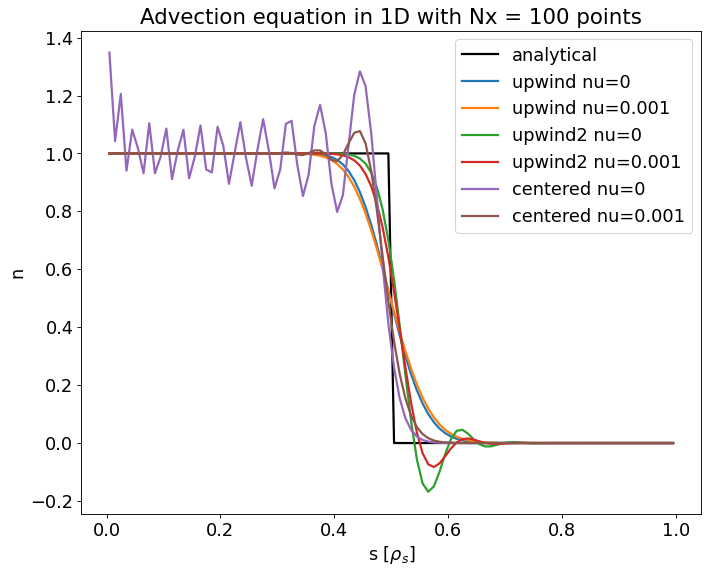
We find the expected results:

the upwind scheme of first order does not produce oscillations and has inherent numerical diffusion
the upwind scheme of 2nd order produces oscillations downstream
the centered scheme without diffusion is unconditionally unstable and produces lots of oscillations
only the first order upwind and the 2nd order schemes with diffusion produce smooth solutions
adding the correct amount of numerical diffusion to the 2nd order schemes depends on the resolution

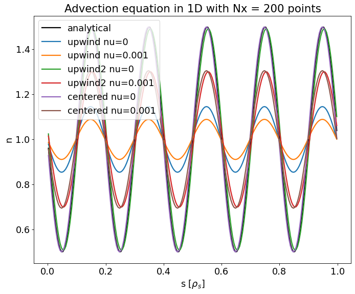
In the wave example we can see that

the upwind scheme of 1st order has a lot of numerical diffusion (even more than the artificial diffusion)
the schemes with diffusion are stable but they do not converge to the correct solution
the 2nd order schemes seem to be stable without diffusion (which is a wrong conclusion as we know that centered differences are unstable, we conclude that the sine wave is not a good test function to test stability)

Navier stokes equation¶

We now turn to the one-dimensional compressional Navier-Stokes equation

(13)¶\[\begin{align} \frac{\partial }{\partial t} n&= - \frac{\partial}{\partial x} (un ) + \nu_n\frac{\partial^2}{\partial x^2} n \\ \frac{\partial }{\partial t} nu&= - \frac{\partial}{\partial x} nu^2 - \alpha\frac{\partial}{\partial x} n^\gamma + \nu_u\frac{\partial^2}{\partial x^2} u \end{align}\]

For \(\gamma=1\) and \(\alpha=\tau\) these are the equations for an ideal gas in 1d, while for \(\gamma=2\) and \(\alpha=0.5g\) we get the shallow water equations.

A numerically particularly challenging initial condition is the Riemann problem

(14)¶\[\begin{align} n(x,0) = \begin{cases} n_l \text{ for } x < x_a \\ n_r \text{ else} \end{cases} \\ u(x,0) = \begin{cases} u_l \text{ for } x < x_a \\ u_r \text{ else} \end{cases} \end{align}\]

For \(\gamma=1\) this leads to Sod’s shock tube problem while for \(\gamma=2\) and \(u_l = u_r = 0\) we have a dam break over a dry/wet bed. Both these cases are widely discussed in the literature and have analytical solutions [DLK+13] for the shallow water case.

We intend to study various schemes to discretize these equations. We will start with the usual naive finite difference approximations on a collocated grid, where both density and velocity are discretized on the same cell-centres. We either use centered differences for all derivatives or an upwind scheme for the advection term in the continuity equation and Burger’s term (keeping centered differences for the wave terms \(-n\partial_x u\) and \(-\alpha \partial_x n^\gamma\)). These are the schemes that we used for our Feltor simulations in the past.

A more robust approach is to use a so-called staggered grid discretization. This is a finite-volume type scheme and the basic idea is to shift the velocity grid by half a grid-point such that the density is given on cell-centres while the velocity is given on the faces. Of the staggered discretizations, a particularly robust one seems to be the one presented in [HLatcheN13] and the PhD thesis of [Gun15] where favourable qualities are shown:

it is positivity preserving
it is shown to satisfy an entropy inequality
it is shock-capturing

The defining features of the scheme is that the pressure term \(\alpha\partial_x n^\gamma\) in the momentum equation is discretized implicitly and that the momenum form is discretized instead of the velocity formulation. This makes the scheme semi-implicit, however the implicit equation can be trivially solved since the density and momentum equations decouple.

We study various variations of the scheme including taking the pressure term explicitly and discretizing the velocity form.

(15)¶\[\begin{align} \frac{\partial }{\partial t} u&= - \frac{\partial}{\partial x} \frac{u^2}{2} - \alpha n^{-1}\frac{\partial}{\partial x} n^\gamma + \nu_un^{-1}\frac{\partial^2}{\partial x^2} u \end{align}\]

There is also a 2nd order formulation using a slope-limiter proposed in [Gun15], which however might be closer to a flux-limter in fact.

As a first example we study the dam break over a dry bed without viscosity

L2 Error norm is 0.003432017556849239  0.011872511687520466
Timesteps for staggered original is 12845.0

L2 Error norm is 0.0009797106735031029  0.00496257128066188
Timesteps for staggered slope-limiter is 15385.0

the original schemes of 1st and 2nd order converge to the correct solution as advertised

L2 Error norm is 0.003432114919925413  0.011872655472057283
Timesteps for staggered explicit is 20224.0

L2 Error norm is 0.0009798384249787998  0.004963092098361188
Timesteps for staggered slope-limiter-explicit is 25724.0

L2 Error norm is 0.025272087713320616  0.08742852957511606
Timesteps for velocity-staggered explicit is 23505.0
L2 Error norm is 0.01905381826559111  0.07438139021783371
Timesteps for upwind is 18459.0

L2 Error norm is 0.019093938425930587  0.07294307772377516
Timesteps for upwind2 is 20948.0

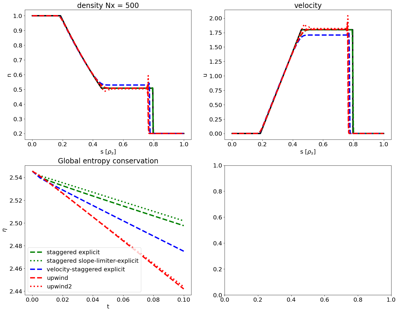
We see that even with very high resolution

the explicit staggered schemes converge to the correct solution as well contradicting the literature; we are unable to reproduce Figure 1.6 in Gunawan’s thesis (even after trying to use fixed-step Euler scheme in order to exclude effects from the different timestepper we use)
the upwind and velocity-staggered schemes both do not converge to the analytic solution

Now we initialize a plane wave in the density and zero velocity. We observe the formation of shocks. Due to Burger’s term the wave crest travels faster than the valley. We investigate the addition of a small viscosity. Since we do not have an analytical solution we treat a high resolution staggered scheme as the true solution:

Timesteps for staggered is 90120.0
Timesteps for staggered slope-limiter-explicit is 49906.0

Timesteps for velocity-staggered explicit is 44577.0

Timesteps for staggered slppe-limiter is 43798.0
Timesteps for upwind is 31852.0

We observe that

shocks can form due to burgers term (the wave top moves faster than the wave bottom, steepening the front)
surprisingly the collocated-upwind scheme is off by quite a bit for the low resolution ( but gets closer for higher resolution and higher viscosity)
for very high resolution (Nx = 1000) all schemes coincide (not shown)
if the viscosity is too small the centered scheme cannot compete (not shown in plot but it is far off)
for the low resolution (Nx = 100) the velocity-staggered scheme seems qualitatively to behave as the staggered schemes, also in the entropy conservation, except for a slightly too large density

Plasma two-fluid equations¶

As a next step we investigate the two-fluid equations (also known as two-fluid Euler-Poisson system)

(16)¶\[\begin{align} \frac{\partial }{\partial t} n_e&= - \frac{\partial}{\partial x} (u_en_e ) + S_{n} \\ \frac{\partial }{\partial t} n_i&= - \frac{\partial}{\partial x} (u_in_i ) + S_{n} \\ \frac{\partial }{\partial t} n_eu_e&= - \frac{\partial}{\partial x} n_eu_e^2 - \frac{\tau_e}{\mu_e}\frac{\partial}{\partial x} n_e - \frac{1}{\mu_e} n_e\frac{\partial}{\partial x} \phi - \frac{\eta}{\mu_e} n_i (n_i u_i - n_e u_e) + \nu_{u,e}\frac{\partial^2}{\partial x^2} u_e\\ \frac{\partial }{\partial t} n_iu_i&= - \frac{\partial}{\partial x} n_iu_i^2 - \frac{\tau_i}{\mu_i}\frac{\partial}{\partial x} n_i - \frac{1}{\mu_i}n_i\frac{\partial}{\partial x} \phi - \frac{\eta}{\mu_i} n_i (n_i u_i - n_e u_e) + \nu_{u,i}\frac{\partial^2}{\partial x^2} u_i \end{align}\]

which is closed by the one-dimensional Poisson equation

(17)¶\[\begin{align} -\frac{\partial^2}{\partial x^2} \phi = \frac{n_i - n_e}{\epsilon_D} \end{align}\]

where we have Gyro-Bohm normalization and \(\mu_e = -m_e/m_i\), \(\mu_i = 1\), \(\tau_e = -1\) and \(\tau_i = T_i / T_e\). Further, we have \(\eta = 0.51 \nu_{ei,0}/ \Omega_{ce}\) and \(\nu_{u,e} = 0.73 \Omega_{ce} / \nu_{ei,0}\) and \(\nu_{u,i} = 0.96 \Omega_{ci} / \nu_{ii,0}\). Last, we have the Debye parameter \(\epsilon_D = \lambda_D^2 / \rho_s^2\) with the Debye length \(\lambda_D\) and the ion gyro-radius at electron temperature \(\rho_s\). Note that we choose the peculiar signs in \(\mu_e\) and \(\tau_e\) such that the electron and ion momentum equations have exactly the same form, which makes it easy to implement.

Also note that we choose Bohm normalization based on gyro-radius \(\rho_s\) and gyro-frequency \(\Omega_{ci}\) because this is how we normalize the three-dimensional model. However, there is no magnetic field in the model and so the gyration does not appear. The more natural normalisation uses plasma frequency and Debye length, which makes the \(\epsilon_D\) parameter disappear [SS87].

The spatial domain is given by \([-L_\parallel /2 ; L_\parallel/2]\), where \(L_\parallel = 2\pi q R_0\) with \(q=3\) and \(R_0=0.545\)m approximating the length of a fieldline from divertor to divertor in the Compass SOL. We use \(N_x\) points.

Neutral fluid limit¶

We reach the limit of Navier Stokes fluid equations by first setting \(\mu_e = 0\). Then we find from the electron momentum equation \(-\tau_e \partial_x n_e - n_e\partial_x \phi - \eta n_e j = 0\), which yields the force term \(-\tau_i \partial_x n_i + \tau_e \partial_x n_i + \tau_e \epsilon_D \partial_x^3 \phi + \epsilon_D \partial_x (\partial_x \phi)^2 / 2 \) in the ion momentum equation. In the limit \(\epsilon_D=0\) the ion continuity and ion momentum equations thus decouple from the system and yield the Navier Stokes equations.

Adiabatic electrons¶

In the limit of \(\mu_e=0\) and vanishing resistivity \(\eta =0\) the electron force balance reduces to \(\partial_x n_e = n_e \partial_x\phi\) which is solved by \(n_e = n_{e,0}\exp(\phi)\).

(18)¶\[\begin{align} \frac{\partial }{\partial t} n_i&= - \frac{\partial}{\partial x} (u_in_i ) + S_{n} \\ \frac{\partial }{\partial t} n_iu_i&= - \frac{\partial}{\partial x} n_iu_i^2 - \tau_i\frac{\partial}{\partial x} n_i - n_i\frac{\partial}{\partial x} \phi + \nu_{u,i}\frac{\partial^2}{\partial x^2} u_i \end{align}\]

which is closed by the one-dimensional non-linear Poisson equation (choosing \(n_{e,0}=1\))

(19)¶\[\begin{align} -\frac{\partial^2}{\partial x^2} \phi = \frac{n_i - \exp(\phi)}{\epsilon_D} \end{align}\]

First, we simulate the full plasma two-fluid system.

Timesteps for staggered original is 725.0

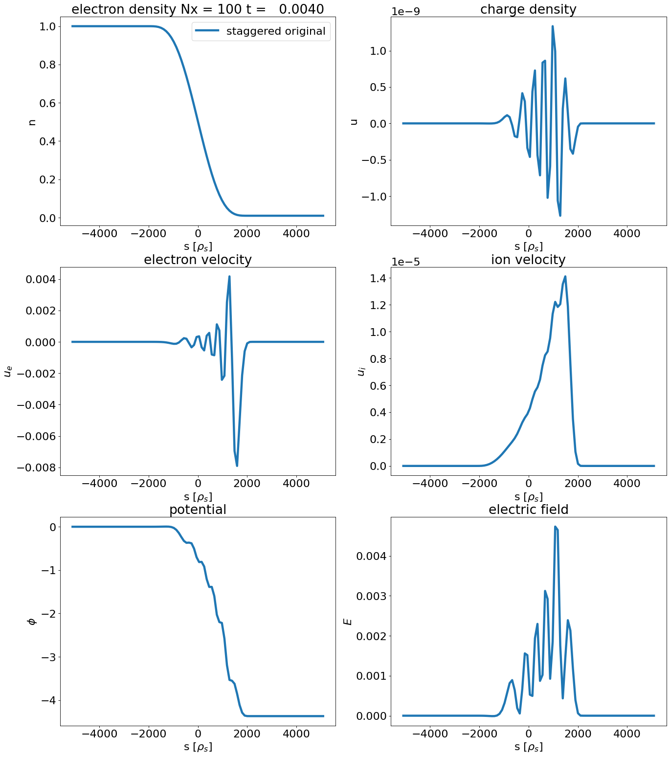
We observe

steps in the potential
oscillations in the electron velocity and electric field indicating rapid plasma oscillations

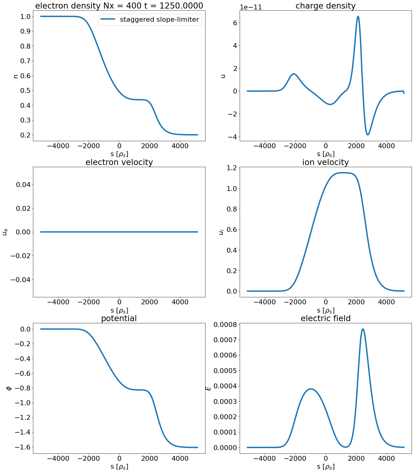
Timesteps for staggered slope-limiter is 20552.0

staggered original 100 5.580296254580168e-05	0.023195936061266877	0.002575918155506441

staggered original 200 2.8282088300430025e-05	0.011705288819374821	0.0011112195383459545

staggered original 400 1.4233827548520823e-05	0.005877695490863391	0.0005277675970782922
staggered slope-limiter 100 1.090675926467633e-05	0.001976291856643779	0.001339650743226408

staggered slope-limiter 200 2.727761445330482e-06	0.0004996362259588693	0.00033494442001343896

staggered slope-limiter 400 6.808894613093873e-07	0.0001251456288766868	8.376258715632446e-05
staggered slope-limiter-explicit 100 1.0905408903246603e-05	0.001972221786447545	0.0013370735038095336

staggered slope-limiter-explicit 200 2.7259884698560088e-06	0.0004987128193436745	0.00033426421736756337

staggered slope-limiter-explicit 400 6.782599516324007e-07	0.00012512265402499096	8.355670477792765e-05
centered 100 2.8162603120836513e-06	0.002525936373990322	0.006341152712926746

centered 200 7.068546265656482e-07	0.0006277146840703361	0.0015818941194588863

centered 400 1.769526754020677e-07	0.00015676610885135612	0.00039538234986413485

%matplotlib inline

Discontinuous Galerkin methods