Matrix free solvers
Contents
Matrix free solvers#
Elliptic equation#
We here study the general two-dimensional elliptic equation
which in a two-dimensional Cartesian grid reads
The task is to find a solution for \(\phi\) for given \(\rho\) and \(\chi\).
Discretization#
We use discontinuous Galerkin (dG) methods to discretize
where \(D_x\) is a block-sparse matrix. We then have
We here see that \(M\) is self-adjoint, which means that we can use a conjugate gradient (CG) solver.
Problem#
// Pseudo-code:
Grid g;
Matrix dx = create_dx (g, bcx), dy = create_dy(g, bcy), j = create_jump();
DiagMatrix diag_chi = create_from_given_vector(chi);
// assembly of M requires four matrix-matrix multiplications and 2 additions
Matrix M = dx.transpose()*diag_chi*dx + dy.transpose()*diag_chi*dy + j;
// Now solve with CG
CG cg;
Vector phi = discretize_phi(g), rho = discretize_rho(g);
cg.solve( M, phi, rho, eps = 1e-8);
In order to assemble \(M\) four matrix-matrix multiplcations need to be performed
This takes longer than the entire CG solve, at least in our initial tests (admittedly 10 years ago)
Solution: matrix - free solvers#
Matrix-free
A matrix-free solver is any solver for \(M x = b\) that does not require access to the elements of the matrix \(M_{ij}\)
Matrix-free solvers are thus a subclass of available solvers
Examples of solvers that are matrix-free:
All Krylov-subspace solvers are matrix-free. E.g. conjugate gradient (CG), LGMRES, BICG, etc.
Fixed point iterations
Chebyshev iteration
Examples of solvers that are not matrix-free
Direct solvers; need to access \(M_{ij}\) directly
Jacobi iteration; because it needs to decompose \(M = D + L + U\)
Gauss-Seidel iteration; needs to decompose \(M = L_* + U\)
Example: Main loop of CG algorithm#
To solve
the main loop of CG reads https://en.wikipedia.org/wiki/Conjugate_gradient_method
To implement you only need to implement the application of \(M\) to a vector rather than \(M\) itself
Grid g;
Matrix dx = create_dx (g, bcx), dy = create_dy(g, bcy), j = create_jump();
DiagMatrix diag_chi = create_from_given_vector(chi);

// Implement the effet of matrix without ever assembling it
Vector matrix_vector_product_with_elliptic_matrix( Vector phi)
{
    Vector dxP = dx*phi, dyP = dy*phi, JP = j*phi;
    Vector tempX = diag_chi*dxP, tempY = diag_chi*dyP;
    dxP = dx.transpose()*tempX, dy= dy.transpose()*tempY;
    return dxP + dyP + JP;
}

// In main CG loop
Vector Ap= matrix_vector_product_with_elliptic_matrix( p_k);
double alpha = r_old / p*Ap;
x = x + alpha*p;
r = r - alpha*Ap;
r_new = r*r;
double beta = r_new/r_old;
p = r + beta*p;
r_old = r_new;
A manufactured example problem#
We manufacture the solution
for \(A\in ]-1,1[\) and solve on the domain \([0,\pi]\times [0,2\pi]\) for Dirichlet boundary conditions in \(x\) and periodic in \(y\). The initital guess is zero.
Interface to Feltor from python#
We have a C++ program “solvers.cpp” written using the FELTOR library.
Takes json file as input
Writes output as yaml
import simplesimdb  # A leightweight data creator and database manager
import numpy as np
import pandas as pd
import matplotlib.pyplot as plt
import yaml # for output files

pd.set_option('display.float_format', lambda x: '%.2e' % x)
# Type make solvers in the repository to have the executable available
database = simplesimdb.Manager( executable='./solvers', directory='data', filetype = 'yaml')
Create some default input parameters#
def create_solver() :
    return {
        "type" : "CG", # CG, LGMRES, BICGSTABl, Multigrid
        "eps" : 1e-6,
        "preconditioner" :{
            "type" : "none" # None or diagonal
        },
        "max_iter" : 50000, # maximum number of iterations
        # for CG
        "check-every" : 1, # errror check every .. iterations
        # for LGMRES
        "inner_m" : 30,
        "outer_k" : 3,
        # for BICGSTABL
        "l_input" : 3
    }
def create_inputfile ():
    '''Create an input file for the solvers FELTOR code'''
    return {
        "grid" : {
            "n" : 3,
            "Nx" : 128,
            "Ny" : 256,
        },
        "solver" : create_solver(),
        "equations":
        {
            "amp" : 0.9, # The closer to 1 the more difficult!
        },
        "elliptic" :
        {
            "jfactor" : 1,
            "direction" : "forward" # forward or centered

        }
    }
Some basic setup#
# Clean out all existing simulations
database.delete_all()
database.directory='data'
def make_dataframe():
    '''Make a pandas Dataframe of all simulations in the database

    Concatenates all inputs and outputs as serialized dicts
    '''
    inputs  = list()
    outputs =list()
    for data in database.table() :
        inputs.append( data)
        with open( database.outfile( data)) as f:
            output = yaml.full_load(f)
            outputs.append( output)
    dfi = pd.json_normalize(inputs)
    dfo = pd.json_normalize(outputs)
    return pd.concat([dfi, dfo], axis=1).sort_values( 'time', ascending=False)
Our first solver test: Unpreconditioned CG on a Nvidia Titan Xp#
# Create an inputfile
inputfile = create_inputfile()

# Run a simulation
outputfile=database.create( inputfile)

# Read in the outputfile (yaml in this case)
with open(outputfile) as f:
    output = yaml.full_load(f)

# Print
print(inputfile)
print(output)
Running simulation 2c3fd2...d15a.yaml
{'grid': {'n': 3, 'Nx': 128, 'Ny': 256}, 'solver': {'type': 'CG', 'eps': 1e-06, 'preconditioner': {'type': 'none'}, 'max_iter': 50000, 'check-every': 1, 'inner_m': 30, 'outer_k': 3, 'l_input': 3}, 'equations': {'amp': 0.9}, 'elliptic': {'jfactor': 1, 'direction': 'forward'}}
{'time': 1.43784, 'iter': 4133, 'error': 8.07962e-08, 'error_abs': 1.79484e-07}
Let us print this in a nicer way#
# Use Pandas to analyse the data in a nice way
df = make_dataframe()
df[['solver.type','solver.preconditioner.type','grid.n','grid.Nx','grid.Ny','iter','time']]
| solver.type | solver.preconditioner.type | grid.n | grid.Nx | grid.Ny | iter | time | |
|---|---|---|---|---|---|---|---|
| 0 | CG | none | 3 | 128 | 256 | 4133 | 1.44e+00 |
Preconditioners in a matrix-free solver#
Problem: since the matrix elements are un-known the preconditioner also needs to be matrix-free
We guess:
Diagonal preconditioner
inputfile = create_inputfile()
inputfile["solver"]["preconditioner"]['type'] = 'diagonal'

database.create( inputfile)

df = make_dataframe()
df[['solver.type','solver.preconditioner.type','grid.n','grid.Nx','grid.Ny','iter','time']]
Running simulation 2e0250...195b.yaml
| solver.type | solver.preconditioner.type | grid.n | grid.Nx | grid.Ny | iter | time | |
|---|---|---|---|---|---|---|---|
| 0 | CG | none | 3 | 128 | 256 | 4133 | 1.44e+00 |
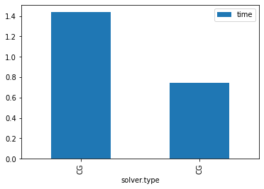
| 1 | CG | diagonal | 3 | 128 | 256 | 2097 | 7.41e-01 |
ax = df.plot.bar(x='solver.type',y="time")
How do other Krylov-solvers fare against CG?#
LGMRES#
inputfile = create_inputfile()
inputfile["solver"]["preconditioner"]['type'] = 'diagonal'
inputfile["solver"]["type"] = "LGMRES"

database.create( inputfile)
# df = make_dataframe()
# df["time_per_iter"] = df["time"]/df["iter"]
# dff = df[['solver.type','solver.preconditioner.type','grid.n','grid.Nx','grid.Ny',
#           'iter','time','time_per_iter','error']]
# dff
Running simulation 125aff...937d.yaml
'data/125afff62b1d961512876210dda326f55d55937d.yaml'
BICGSTABl#
inputfile = create_inputfile()
inputfile["solver"]["preconditioner"]['type'] = 'diagonal'
inputfile["solver"]["type"] = "BICGSTABl"

database.create( inputfile)

df = make_dataframe()
df['time_per_iter'] =  df["time"]/df["iter"]
dff = df[['solver.type','solver.preconditioner.type','grid.n','grid.Nx','grid.Ny','iter','time','time_per_iter']]
dff
Running simulation 22c9a0...3d3d.yaml
| solver.type | solver.preconditioner.type | grid.n | grid.Nx | grid.Ny | iter | time | time_per_iter | |
|---|---|---|---|---|---|---|---|---|
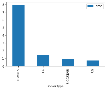
| 0 | LGMRES | diagonal | 3 | 128 | 256 | 5229 | 7.92e+00 | 1.51e-03 |
| 2 | CG | none | 3 | 128 | 256 | 4133 | 1.44e+00 | 3.48e-04 |
| 1 | BICGSTABl | diagonal | 3 | 128 | 256 | 1374 | 9.38e-01 | 6.82e-04 |
| 3 | CG | diagonal | 3 | 128 | 256 | 2097 | 7.41e-01 | 3.53e-04 |
ax = df.plot.bar(x='solver.type',y="time")
Observations#
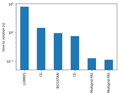
LGMRES is almost a factor 10 worse than CG for this problem (other problems may have different results)
BICGSTABl fares almost as well as normal CG
Matrix-free (geometric) multigrid#
Classical multigrid consists of three ingredients [Briggs, W.L., Henson, V.E., and McCormick, S.F. (2000) A multigid tutorial]
A grid restriction/prolongation
A (direct) solver on the coarsest grid
A smoother on the other grids
With matrix-free (dG) solvers:
restriction/prolongation is straightforward
A direct solver is inadmissable
Most smoothers (e.g. Gauss-Seidel) are not matrix-free
A first attempt: Nested iterations#
IDEA:
project initial guess to coarsest grid
solve with PCG up to accuracy
interpolate solution to next fine grid
solve with PCG (with interpolated solution as initial guess)
…
This employs ideas from “Full approximation scheme” and also works for nonlinear problems
[Van Emden Henson “Multigrid methods for nonlinear problems: an overview”, Proc. SPIE 5016, Computational Imaging, (1 July 2003);]
def create_multigrid_inputfile():
    return {
        "grid" : {
            "n" : 3,
            "Nx" : 128,
            "Ny" : 256,
        },
        "solver" :
        {
            "type" : "Multigrid-FAS", # Full approximation scheme
            "num_stages" : 3,
            "solvers" :
            [
                create_solver(), # Solver on stage 0 (the fine grid)
                create_solver(), # Solver on stage 1 (the next grid)
                create_solver()  # Solver on stage 2 (the coarse grid)
            ]
        },
        "equations":
        {
            "amp" : 0.9, # The closer to 1 the more difficult
        },
        "elliptic" :
        {
            "jfactor" : 1,
            "direction" : "forward" # forward or centered

        }
    }
inputfile = create_multigrid_inputfile()
for i in (0,1,2):
    inputfile['solver']['solvers'][i]['preconditioner']['type'] = 'diagonal'
inputfile['solver']['preconditioner'] = {'type': 'diagonal'}

database.create( inputfile, error = 'display')
df = make_dataframe()
df["time_per_iter"] = df["time"]/df["iter"]
dff = df[['solver.type','solver.preconditioner.type','grid.n','grid.Nx','grid.Ny',
          'iter','time','time_per_iter', 'error']]
dff
Running simulation 217afd...fdd7.yaml
| solver.type | solver.preconditioner.type | grid.n | grid.Nx | grid.Ny | iter | time | time_per_iter | error | |
|---|---|---|---|---|---|---|---|---|---|
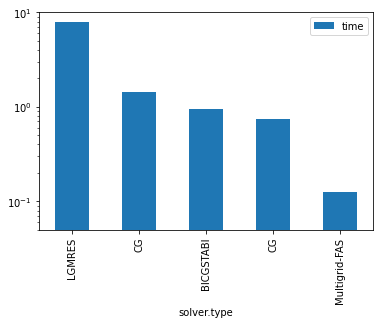
| 0 | LGMRES | diagonal | 3 | 128 | 256 | 5229 | 7.92e+00 | 1.51e-03 | 7.28e-07 |
| 3 | CG | none | 3 | 128 | 256 | 4133 | 1.44e+00 | 3.48e-04 | 8.08e-08 |
| 2 | BICGSTABl | diagonal | 3 | 128 | 256 | 1374 | 9.38e-01 | 6.82e-04 | 1.05e-06 |
| 4 | CG | diagonal | 3 | 128 | 256 | 2097 | 7.41e-01 | 3.53e-04 | 8.23e-08 |
| 1 | Multigrid-FAS | diagonal | 3 | 128 | 256 | 76 | 1.26e-01 | 1.66e-03 | 8.34e-08 |
ax = df.plot.bar(x='solver.type',y="time")
ax.set_yscale('log')
ax.set_ylim([0.05,10])
plt.show()
Fine-tuning: Avoiding scalar products on coarse grid#
On a cluster the most time-consuming operation is the scalar product on the coarse grid. Avoid error check at every iteration.
inputfile = create_multigrid_inputfile()
for i in (0,1,2):
    inputfile['solver']['solvers'][i]['check-every'] = 10 # only check error at every 10-th iteration
    if( i==0 ) :
        inputfile['solver']['solvers'][i]['check-every'] = 1
    inputfile['solver']['solvers'][i]['preconditioner']['type'] = 'diagonal'
    inputfile['solver']['preconditioner'] = {'type': 'diagonal'}
database.recreate( inputfile, error = 'display')
# database.delete( inputfile)
df = make_dataframe()
df["time_per_iter"] = df["time"]/df["iter"]
dff = df[['solver.type','solver.preconditioner.type','grid.n','grid.Nx','grid.Ny',
          'iter','time','time_per_iter','error']]
dff
Running simulation 27f4bd...be14.yaml
| solver.type | solver.preconditioner.type | grid.n | grid.Nx | grid.Ny | iter | time | time_per_iter | error | |
|---|---|---|---|---|---|---|---|---|---|
| 0 | LGMRES | diagonal | 3 | 128 | 256 | 5229 | 7.92e+00 | 1.51e-03 | 7.28e-07 |
| 4 | CG | none | 3 | 128 | 256 | 4133 | 1.44e+00 | 3.48e-04 | 8.08e-08 |
| 2 | BICGSTABl | diagonal | 3 | 128 | 256 | 1374 | 9.38e-01 | 6.82e-04 | 1.05e-06 |
| 5 | CG | diagonal | 3 | 128 | 256 | 2097 | 7.41e-01 | 3.53e-04 | 8.23e-08 |
| 1 | Multigrid-FAS | diagonal | 3 | 128 | 256 | 76 | 1.26e-01 | 1.66e-03 | 8.34e-08 |
| 3 | Multigrid-FAS | diagonal | 3 | 128 | 256 | 76 | 1.11e-01 | 1.46e-03 | 8.22e-08 |
ax = dff.plot.bar(x='solver.type',y="time")
# ax.set_xticklabels(["LGMRES","BICGSTABl","CG (no precond.)", "CG (with precond.)"
# ,"FAS (default)",  "FAS (optimized)"])
ax.set_xlabel( "")
ax.set_yscale('log')
ax.set_ylabel( 'time to solution [s]')
ax.set_ylim([0.05,10])
ax.legend().remove()
# plt.savefig( 'solvers.png', bbox_inches="tight")
plt.show()
Matrix-free Full multigrid#
Matrix-free Full multigrid is possible using
use Chebyshev iterations as smoother
use CG on coarse grid as solver
BUT
no performance improvement over nested iterations (in our tests)
sometimes does not converge at all
Conclusions#
Matrix-free solvers avoid assembly cost of matrix
CG solver can have large speedup (up to 10x) over LGMRES for symmetric problems
Matrix-free multigrid possible and large speedup (another 10x) over non-multigrid
