Analysis of the dx and dy routines
Contents
Analysis of the dx and dy routines
import numpy as np
from collections import OrderedDict as odict
import pandas as pd
import matplotlib.pyplot as plt
import matplotlib.cm as cm
As done previously, we list the files we want to analyse and setup the plots
#(hardware name, number of nodes, plotstyle)
filesCPUs = {
         'knl_mpi1':('knl',1), 'knl_mpi2':('knl',2), 'knl_mpi4':('knl',4),
         'skl_mpi1':('skl',1), 'skl_mpi2':('skl',2), 'skl_mpi4':('skl',4),
         'i5':('i5',1)
}
filesGPUs = {
         'p100nv_mpi1':('p100',1), 'p100nv_mpi2':('p100',2), 'p100nv_mpi4':('p100',4),
         'v100nv_mpi1':('v100',1), 'v100nv_mpi2':('v100',2), 'v100nv_mpi4':('v100',4),
         'gtx1060':('gtx1060',1,)
             }
# order by number of nodes to make labeling easier further down
cpuFiles = odict(sorted(filesCPUs.items(), key= lambda t : t[1][1]))
gpuFiles = odict(sorted(filesGPUs.items(), key= lambda t : t[1][1]))
# count number of 1 nodes in dict
number=0
for k,v in cpuFiles.items():
    if v[1]==1: number+=1

arch = {'knl':(cm.Greens,450,0.5,0.33),'skl':(cm.Greys,200,0.5,0.75),'p100':(cm.Blues,550,0.5,0.43),
        'v100':(cm.Purples,850,0.5,0.85),'i5':(cm.Wistia,30,0.5,0.79),'gtx1060':(cm.Oranges,155,0.5,0.70)}
intens={1:0.8, 2:0.6, 4:0.4}
marker={2:'d', 3:'o', 4:'s',5:'p'}
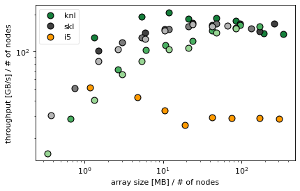
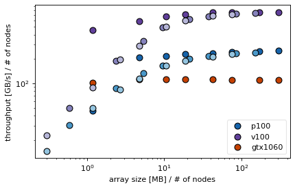
Note that we compute the average bandwidth between the x and y derivative in ‘dxdy’
ns=[3]
for filelist in [cpuFiles, gpuFiles]:
    for q in ['dxdy']:#['dx','dy','dxdy']:
        fig,ax=plt.subplots(1,1,figsize=(6,3.7),dpi= 80, facecolor='w', edgecolor='k')
        for f, v in filelist.items():
            #read in csv file
            df=pd.read_csv('benchmark_'+f+'.csv', delimiter=' ')
            #add size and get rid of non-relevant columns
            df.insert(0,'size', 8*df['n']*df['n']*df['Nx']*df['Ny']/1e6/v[1])
            bw = df[['n','Nx','Ny','size']]
            bw = bw.assign(dx = df['size']/1000*3/df['dx'])#/arch[v[0]][1])
            bw = bw.assign(dy = df['size']/1000*3/df['dy'])#/arch[v[0]][1])
            bw = bw.assign(dxdy=2.0*bw['dx']*bw['dy']/(bw['dx']+bw['dy']))
            #compute mean and standard derivation of 'same' groups
            bw=bw.groupby(['n', 'Nx','Ny','size']).agg(['mean', 'std'])
            bw=bw.reset_index(level=['Nx','Ny','size'])

            for n in ns:
                bwn = bw.loc[n]
                bwn.reset_index(inplace=True)
                toPlot = bwn['dxdy'].join(bwn['size'])
                #print(toPlot)
                toPlot.plot(ax=ax,color=arch[v[0]][0](intens[v[1]]), marker=marker[n],ls='',markeredgecolor='k',
                             x='size',y='mean',label=v[0], markersize=8)
        plt.xlabel('array size [MB] / # of nodes')
        plt.ylabel('throughput [GB/s] / # of nodes')
        plt.xscale('log')
        plt.yscale('log')
        #for k,v in arch.items():
        #    if q=='mixed' :
        #        plt.axhline(y=v[3],xmin=v[2],xmax=1,color=v[0](1.0),lw=2)
        handles, labels = plt.gca().get_legend_handles_labels()
        handles = handles[0:len(ns)*number:len(ns)]; labels = labels[0:len(ns)*number:len(ns)]
        plt.legend(handles, labels, numpoints=1,loc='upper left',
                   fontsize='medium',framealpha=0.5)
        #plt.title(q)
        #plt.ylim(5,1000)
        #plt.xlim(10,1000)
        if filelist == cpuFiles :
            plt.savefig(q+'_cpu.pdf',bbox_inches='tight')
        if filelist == gpuFiles :
            plt.legend(handles, labels, numpoints=1,loc='lower right',
                   fontsize='medium',framealpha=0.5)
            plt.savefig(q+'_gpu.pdf',bbox_inches='tight')


Conclusions
efficiency of derivatives difficult to determine for skl and knl
depends on n (the number of polynomial coefficients)
high latencies for NVidia GPUs make MPI + GPU slow for small to medium sizes (-> calls for nvlink)
also for KNL the latencies in MPI seem very high, in fact MPI seems to be systematically slower than non-MPI also for larger sizes -> is this because MPI does not transfer MCDRAM -> MCDRAM instead copying to DDR4 RAM which is systematically slower than the MCDRAM? (but the inner points all live in MCDRAM don’t they?)